Step 2: Carry Out Optimization
Once above files have been prepared, user is ready to carry out optimization.
Load thermodynamic database file
First of all, the database file (.TDB) containing the phases to be modeled is loaded by click the ![]() icon. This database file defines the model type and model parameters of each phase in the system. The model definition is consistent with the currently accepted format in the CALPHAD society, and the model parameters can be real numbers or variables to be optimized.
icon. This database file defines the model type and model parameters of each phase in the system. The model definition is consistent with the currently accepted format in the CALPHAD society, and the model parameters can be real numbers or variables to be optimized.
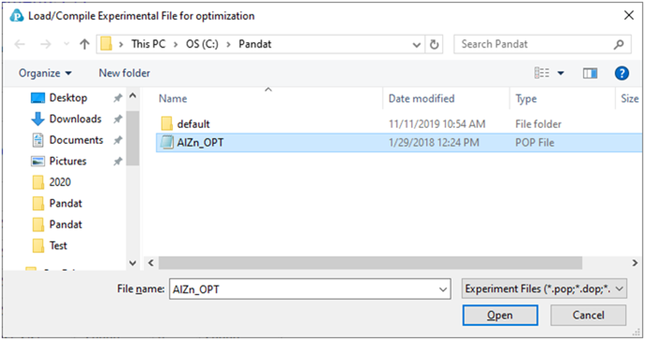
Load and compile experimental file
After loading a TDB file with defined model parameters to be optimized, user should then load and compile the experimental POP file. Go to PanOptimizer menu and choose Load/Compile Experimental File, user can then select the POP file already prepared as shown in Figure 1. User can also choose Append Experimental File to append new experimental data stored in a separate file to the currently opened POP file.
Perform Optimization
Once the TDB file and the experimental POP file are loaded, user is ready to do the optimization. In the current version of PanOptimizer, the optimization is controlled through the optimization control panel as shown in Figure 2. There are four control areas in the optimization control panel. They are: Histogram (A), Bound/Unbound Variables (B), Optimization (C), and Optimization Results (D).
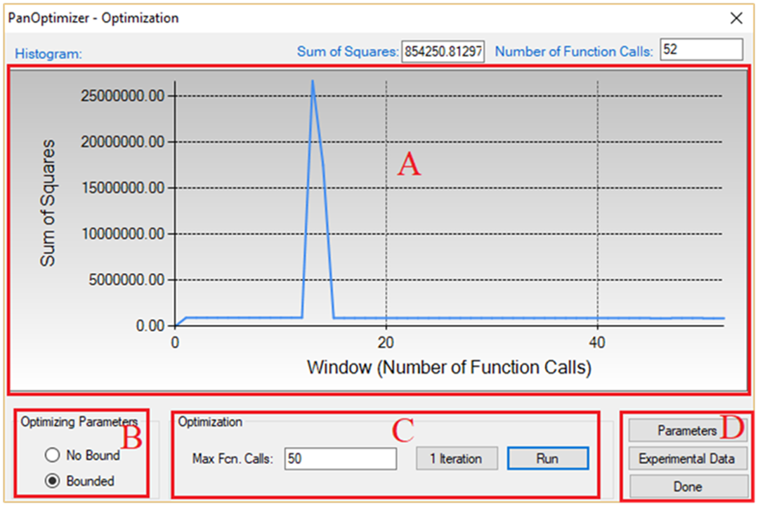
Histogram (A)
Histogram is for displaying and tracing the history of the discrepancy between model-calculated values and experimental data, which is characterized by the Sum of Squares displayed during the whole optimization procedure. The histogram plots the sum of squares vs. the number of function calls. The exact value of the sum of squares in the current step can be found at the up-right corner of this area.
Free Bound/Unbound Variables (B)
The user can choose the model parameters to be optimized in either the bounded or the unbounded mode. In the bounded mode, the low and high bounds defined in a TDB file will take into effects.
Optimization (C)
The goal of the optimization process is to obtain an optimal set of model parameters so that the model calculated results can best fit the given experimental measurements. The optimization process can be controlled by choosing “1 Iteration” or “Run”. With “1 Iteration”, the maximum number of function calls is set to be 2(N + 2), where N is the number of model parameters to be optimized. The user can click “Run” mode several times until the optimal solution is found or the designated maximum number of function calls is reached.
Here we take the binary Al-Zn system as an optimization example. The TDB and POP files are available at the installing directory of Pandat “/Pandat_Examples/PanOptimizer/”. In this example, there are totally 11 parameters to be optimized and all the initial values are set to be zero. The available experimental data include:
-
mixing enthalpy of liquid phase at 953K
-
invariant reaction at 655K: Liquid → Fcc + Hcp
-
invariant reaction at 550K: Fcc#2 → Fcc#1 + Hcp
-
tie-lines: Fcc#1+Fcc#2, Liquid + Fcc, Liquid + Hcp and Hcp + Fcc
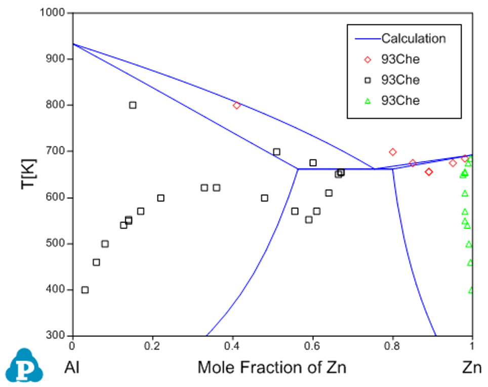
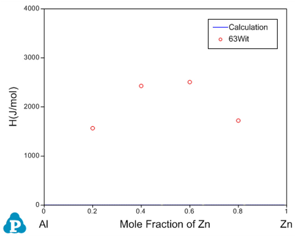
Before the optimization, user may want to check the calculated results using the initial set of model parameters without optimization. Phase diagram calculation can be done through 2-D section calculation, and enthalpy calculation can be done through the 1-D line calculation. Figure 3 shows the calculated Al-Zn phase diagram and enthalpy of mixing for liquid phase at 953K along with the given experimental data, respectively. The parameters before optimization result in large discrepancies between the calculated values and the experimental measurements. Optimization of these model parameters (initially set as zero) is needed.
By clicking “Run” twice (two rounds), and each run performs 50 function calls, the sum of squares decreases from 854251 to 403 as shown in Figure 4(a). After another round of Run, the sum of squares decreases from 403 to 3.15 as shown in Figure 4(b). Now, we can do the real time calculation using the instantly obtained optimized parameters. The two comparisons in Figure 5 show excellent agreements between the calculated results and the measured data. By selecting the command from PanOptimizer menu: “PanOptimizer → Add Exp. Data to the current Graph”, user can add the corresponding experimental data defined in the pop file directly to the calculated diagram for comparison.
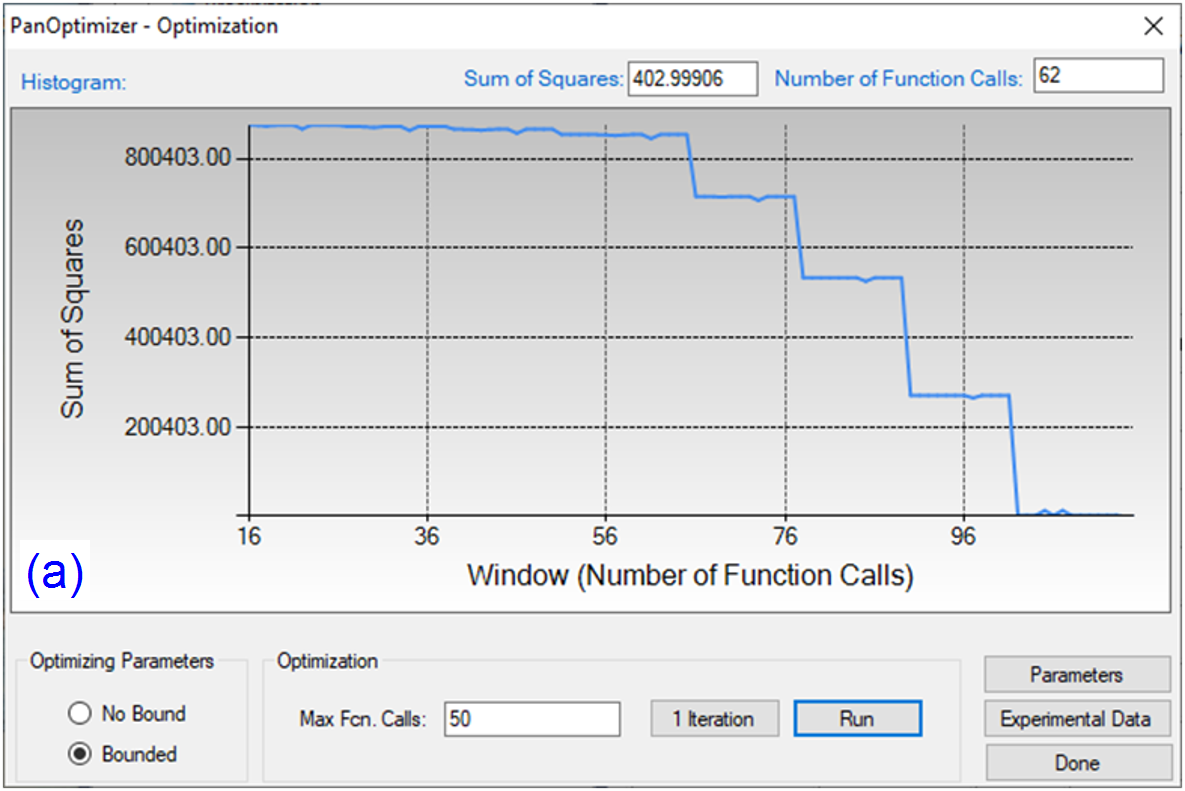
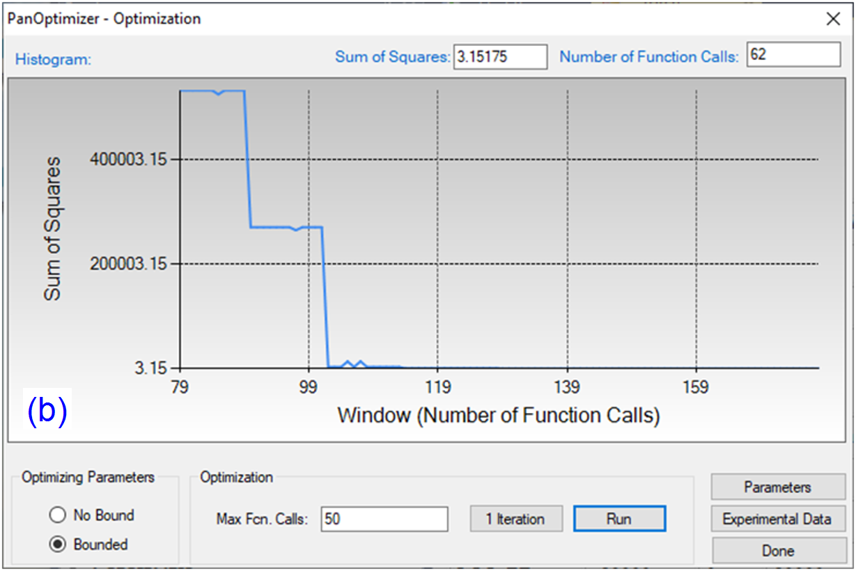
Figure 4: (a) Sum of squares after two rounds of optimization (b) Sum of squares after another two rounds of optimization
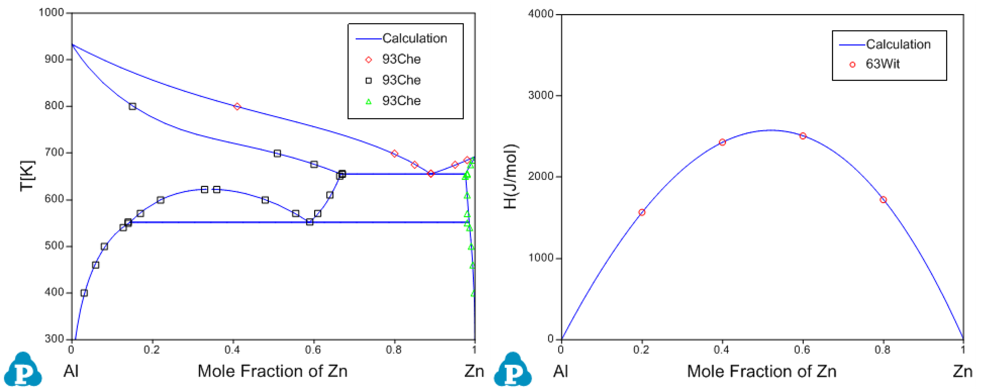
Figure 5: Comparison between the calculated results and the experimental data after optimization
Optimization Results (D)
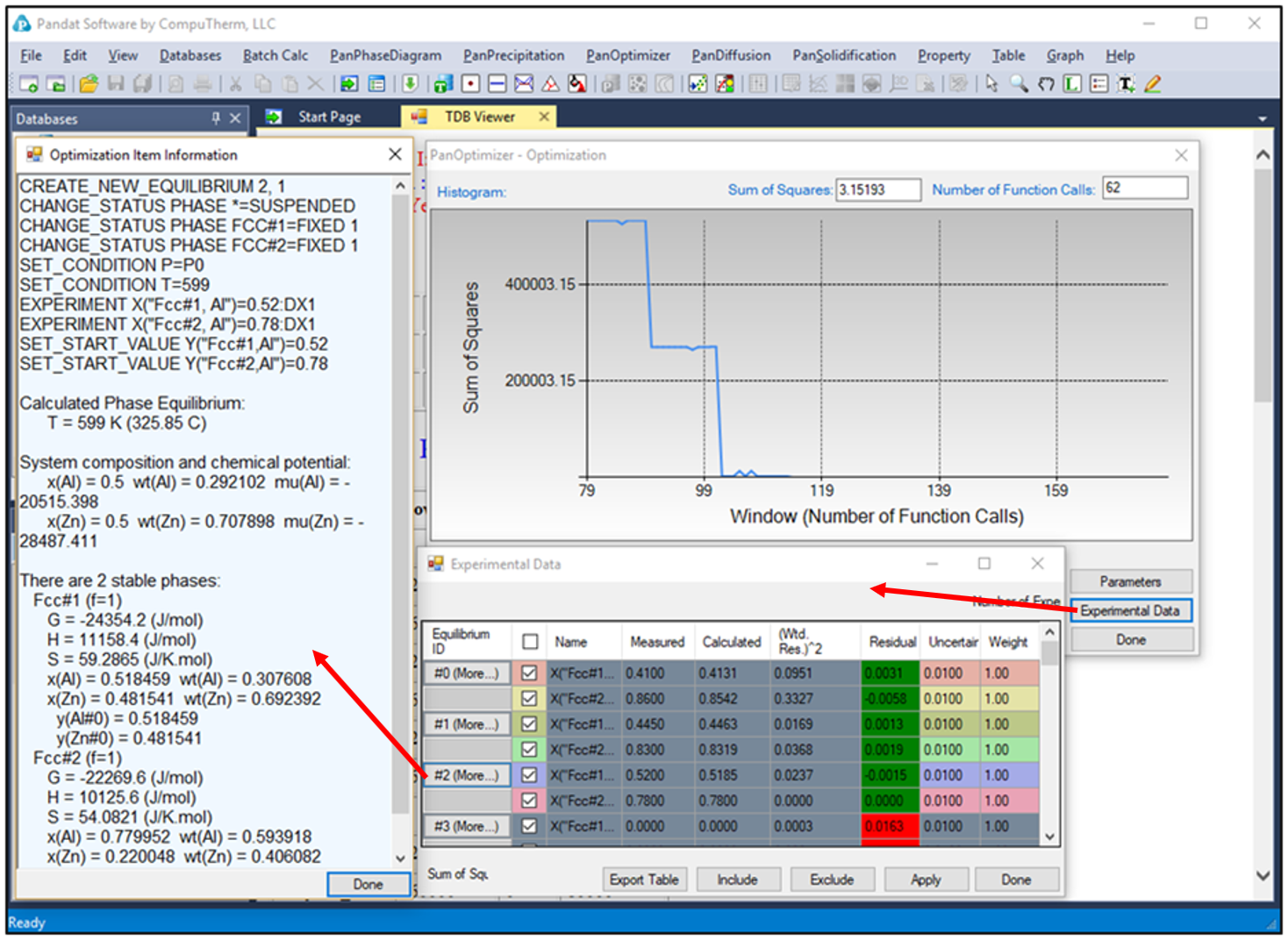
During optimization, user can check model parameters through the Parameters button as shown in Figure 2. For each model parameter, user can change its low bound, upper bound and initial value in the dialog window as shown in Figure 6. User can “Include” or “Exclude” a certain parameter in the optimization through the “check box” in front of the parameter. If a set of optimized parameters is satisfactory, user can save this set of values as default ones through Set Default shown in Figure 6. Otherwise, user can reject this set of values and go back to previous default values through Get Default. User also can save the TDB file with the optimized model parameters through Save TDB. The standard deviation and relative standard deviation (RSD) of each parameter are computed during optimization. The parameter evolution during the last 100 iterations can be tracked by clicking the parameter name in the table as indicated in Figure 6. It should be noted that any changes on model parameters made by user will take into effect only after the button Apply is clicked.
By clicking the “Experimental Data” button onFigure 4(b), a table which lists the calculated values together with the experimental data will pop out as shown in Figure 7. This table allows user to view how well the current optimized parameters describe each set of experimental data. If the discrepancy is found to be large and not satisfied for a certain set of data, a larger weight factor for this set of data can be given in the next round of optimization. Through the column of Residual shown in Figure 7, user can see different color after each comparison. The green means satisfactory results are achieved, while the red color means large deviation remaining. Again, user can Include or Exclude a certain experimental data set for the optimization through the check box in front of each experimental data Name. Also, more detailed experimental data information can be viewed by clicking the Equilibrium ID of the experimental data in the table.